
Megan Langford
Let
us first take a look at the following basic graph:
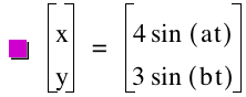
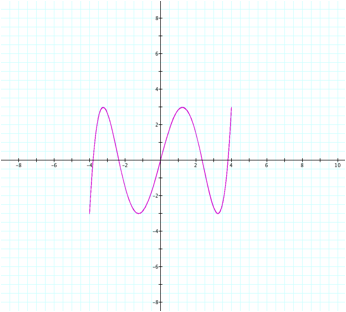
We
will set a=1, b=2, and t=0…30 to start.
We
can now notice several different observations. First, the minimum x value is -4, while the maximum is
4. This directly corresponds to
the coefficient in front of the x= function. We know that this makes sense because the output values of
the sine function range between -1 and 1.
Multiplying these by 4 will give you what we see here in the graph.
Next,
the minimum y value is -3, and the maximum y value is 3. As we now could have guessed, this
directly corresponds to the coefficient in front of the y= function. Again, this is consistent with our
knowledge of the sine function, because its output values when multiplied by 3
would range between -3 and 3.
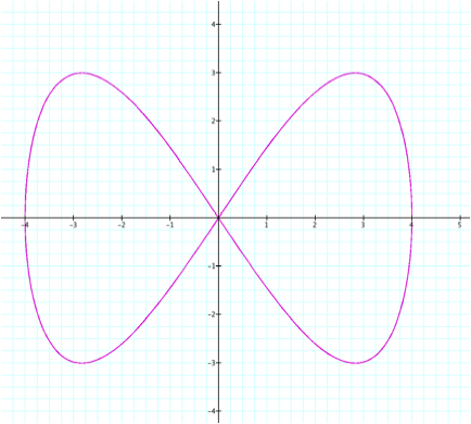
To
further illustrate this behavior, let’s look at another example to show the
behavior remains consistent.
Again, we will keep a=1 and b=2 here.

This
example confirms our conjecture that the corresponding coefficient determines
the range and domain for the function.
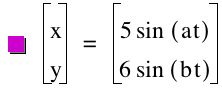
This is because with a coefficient of 5, ![]() , and with a coefficient of 6,
, and with a coefficient of 6, ![]() .
.
In
addition, we can note that there appear to be 2 sections to the graph. By
sections, I mean the number of humps between the x-intercepts as we move from
left to right along the x-axis. We
can hypothesize that perhaps this is the case because b=2. If so, when we choose another value for
b, there should be that number of sections to the graph as well.
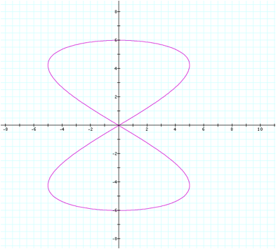
This
time, we will use the same equations in the original function, but we will set
b=6. Will there be 6 sections of
the graph?
Of
course, we can notice the change right away. Rather than having only 2 sections to the graph, we now have
6. To reiterate, we have changed
the b value from 2 to 6. Clearly,
the number of sections appears to have a direct correspondence to the value of
b. However, notice that there is
both a top and a bottom curve for each “section” of the graph. What happens if we choose an odd number
for b? Will this still be the
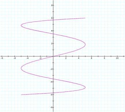
case? Let’s explore when b=5.
Instead
of having a top and bottom to each “section,” the curve only exists for one or
the other in this case. Also, it’s
worth noting that if we used the two tails on either end that extend beyond an
x-intercept and placed them together, we would have our 5th section,
which does uphold our earlier assertion that the number of sections is
determined by the b value.
Now
let’s take a look at how the graph will change if we set the a value to be
larger than the b value. Here,
let’s let a=2 and b=1.
We
can immediately notice that the graph appears to be very similar to our earlier
graph where a=1 and b=2, except that rather than being oriented at the x-axis,
this one is oriented at the y-axis.
We could say the graph almost appears to have rotated 90 degrees.
Additionally,
we can notice that this graph retains the same intervals for the domain and
range that our second graph did.
The y values remain in the interval ![]() , and the x values remain in the interval
, and the x values remain in the interval ![]() . This is
because these intervals are still being determined by the coefficients before
the trigonometric functions in each case, which we have kept the same between
the two graphs.
. This is
because these intervals are still being determined by the coefficients before
the trigonometric functions in each case, which we have kept the same between
the two graphs.
Finally,
we can experiment with different a values like we did with the b values to see
how the changes will affect the shape of the graph. Let’s look at the graph when a=6 and b=1. Will we end up with 6 sections of the
graph like we did when b=6 and a=1?
Indeed,
this is the case. The domain and
range have remained the same, but the number of sections of the graph have
changed, similar to our 3rd graph.
Then
what will happen if we change the a value to be odd? Will we end up with the same shape we had when b was
odd? Let’s test this by setting
a=5 and b=1.

Indeed,
this graph is quite similar in shape to our 4th graph when we had
set a=1 and b=5. Again, rather
than being oriented horizontally, our newer graph is oriented vertically, since
the a value is larger than the b value.
The sections are not closed since a is an odd number. These observations have held consistent
every time we have changed the coefficient value, a value, and b value for each
graph.
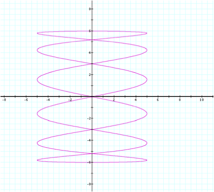
For
some extreme instances of these graphs, here are a few graphs with
exceptionally large a and b values.
When
a=50 and b=1:
When
a=70 and b=200:
When
a=50 and b=200:
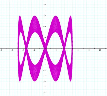
When
a=50 and b=50:
One
final observation we can see clearly demonstrated in the last two graphs is
that if either the a or b value is a multiple of the other, this will affect
the number of sections in the graph.
For example, since ![]() , when a=50 and b=200 (or vice versa) there are only 4 total
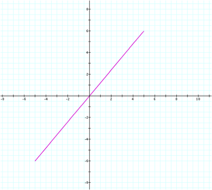
sections. Thus, when a=b, we have
only a straight line and no sections as we did before.
, when a=50 and b=200 (or vice versa) there are only 4 total
sections. Thus, when a=b, we have
only a straight line and no sections as we did before.